
Have you ever tried to explain something complex to a friend? Well, that’s kind of what autoencoders do - they take a big, complicated set of data and try to simplify it into a smaller, more manageable representation. It’s like trying to summarize a 500-page novel into a tweet. Autoencoders consist of two main components: encoder and decoder. In the previous example, the encoder is you that takes the original data and compresses it into a lower-dimensional representation (from novel to a tweet), while the decoder is your friend that takes that compressed data and tries to reconstruct the original input.
So let’s dive in and explore a piece of the world of autoencoders and let’s try to do some magic tricks morphing a number.
Encoders, Decoders and Applications
Autoencoders are two neural network models: encoder and decoder.
Encoders transform input data into a smaller representation called code or latent space. Decoders take as input the latent space and try to convert it into the original data.
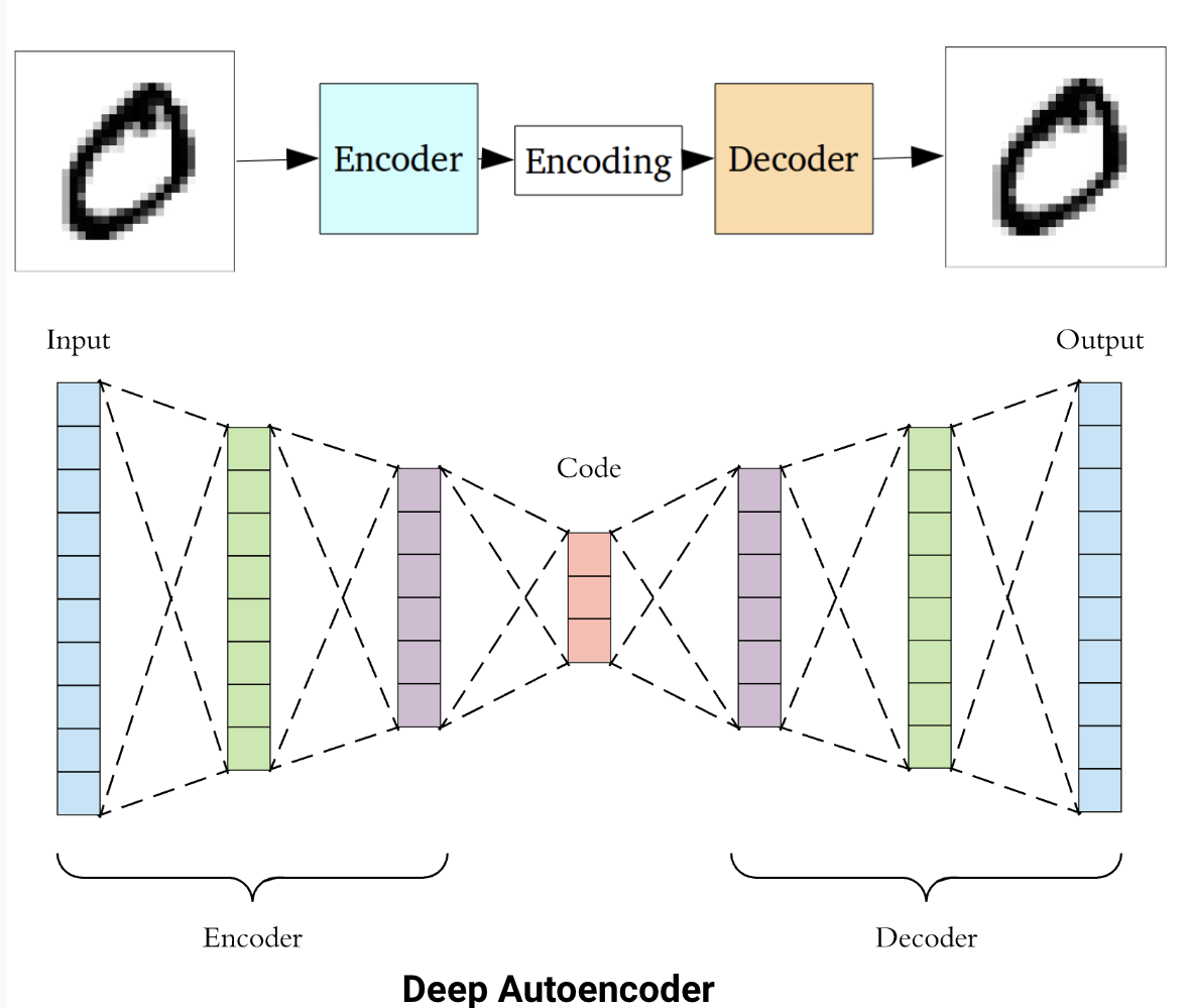
Autoencoders have a wide range of applications. One popular use of autoencoders is in image compression, where the encoder compresses high-dimensional image data into a low-dimensional representation, and the decoder reconstructs the image from that compressed representation. Autoencoders can also be used for feature extraction in image classification tasks. By training an autoencoder to reconstruct images with a bottleneck layer, the network learns to extract the most important features from the original image.
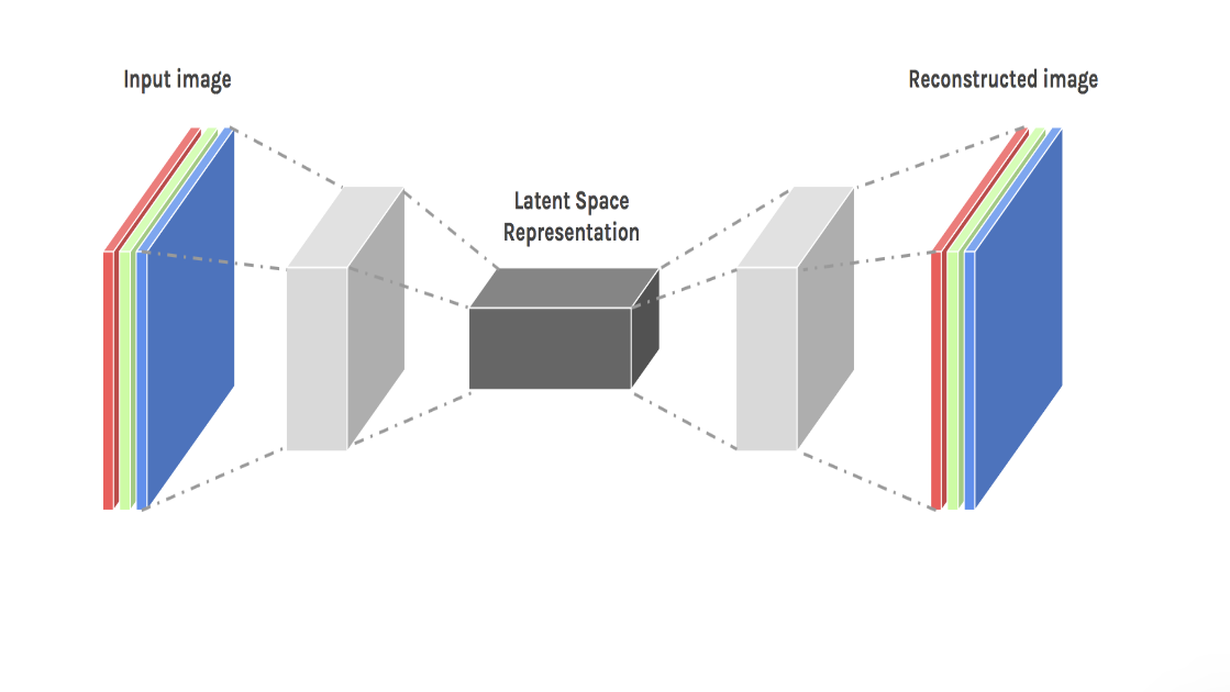
In natural language processing, autoencoders can be used for tasks such as text summarization and language translation. Training an autoencoder to reconstruct a shorter summary of a longer text, the network learns to identify the most important information in the original text.
Finally, autoencoders can also be used for image upscaling. In image upscaling, the goal is to increase the size of a low-resolution image while improving its visual quality.
To perform image upscaling using autoencoders, a low-resolution image is first fed into the encoder, which compresses the image into a lower-dimensional representation. The compressed image is then fed into the decoder, which attempts to reconstruct the original image at a higher resolution. The decoder is trained on a dataset of high-resolution images to learn how to fill in the missing details and create a visually pleasing result.

In this blog, we will explore 2 application of autoencoders:image upscaling and image morphing. We will use a special type of autoencoder: variational autoencoder (VAE), to upscale an image by first compressing it into a low-dimensional representation using the encoder, and then generating a new, higher-resolution image from that representation using the decoder. We will then explore how VAEs can be used to morph one image into another, by first encoding both images into their low-dimensional representations, and then smoothly interpolating between those representations to create a series of new images that gradually blend the two original images.
VAE
Unlike traditional autoencoders, which learn a deterministic mapping from the input to the encoded representation, variational autoencoder learn a probabilistic distribution over the encoded representation. This allows VAEs to generate new, similar representations of the input data.

Specifically, the encoder maps the input image to the mean and variance of a multivariate Gaussian distribution over the latent code. The decoder then samples from this distribution to generate a new latent code, which is used to generate the output image. Basically training a VAE involves minimizing a loss function that consists of two components: a reconstruction loss, which measures the difference between the input image and the output image, and a regularization loss, which encourages the learned distribution over the latent code to match a prior distribution, such as a unit Gaussian. The regularization loss is the core of the VAE that helps prevent overfitting and encourages the VAE to learn a smooth, continuous latent space.
Together, the reconstruction and regularization loss are like a dynamic duo, working hand-in-hand to ensure our network produces high-quality outputs without overfitting. Without them, our network might produce outputs that look nothing like the original input.

Mnist upscale and morphing
The following section desctibe how to upscale and morph the images of MNIST digits classification dataset. I used the coolab notebook with GPU runtime to train my model. I chose to use Google Colab this time because it is a free and because in my last project, I spent a fortune on Azure. So, this time let’s go with a more economical option.
Dataset
Let’s start importing the dataset and scaling the images
1
2
3
4
5
6
7
8
9
10
num_classes = 10
input_shape = (28, 28, 1)

# Load the data and split it between train and test sets
(high_digit_train, train_label), (high_digit_test, test_label) = keras.datasets.mnist.load_data()

# Scale images to the [0, 1] range
y_train = high_digit_train.astype("float32") / 255
# Make sure images have shape (28, 28, 1)
y_train = np.expand_dims(y_train, -1)
Now we need to downscale the images to create the dataset having as input low-resolution images and as output the high-resolution images.
1
2
3
4
5
6
7
8
9
small_size = (8,8)

x_train = tf.keras.preprocessing.image.smart_resize(
    y_train, small_size, interpolation='bilinear'
)

print("x_train shape:", x_train.shape)
print("y_train shape:", y_train.shape)
print(y_train.shape[0], "train samples")
1
2
3
x_train shape: (60000, 8, 8, 1)
y_train shape: (60000, 28, 28, 1)
60000 train samples
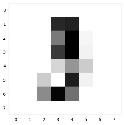
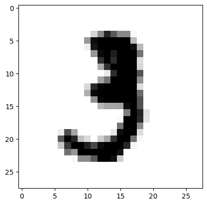
So our dataset is composed by 60000 images where input images are 8x8 pixel images and out images are 28x28 images.
Let’s display some data:
1
2
3
4
5
6
7
i = 10
print("Low resolution")
plt.imshow(x_train[i],cmap=plt.cm.gray_r)
plt.show()
print("High resolution")
plt.imshow(y_train[i],cmap=plt.cm.gray_r)
plt.show()
Low resolution image:
High resolution image:
Model
For the model I used the structure of the VAE model of keras examples and I modified a little bit for our purpose.
The first piece of the model is the Sampling function: the function that given the mean and variance vectors return the latent space:
1
2
3
4
5
6
7
8
9
class Sampling(layers.Layer):
    """Uses (z_mean, z_log_var) to sample z, the vector encoding a digit."""

    def call(self, inputs):
        z_mean, z_log_var = inputs
        batch = tf.shape(z_mean)[0]
        dim = tf.shape(z_mean)[1]
        epsilon = tf.keras.backend.random_normal(shape=(batch, dim))
        return z_mean + tf.exp(0.5 * z_log_var) * epsilon
Then, we need to define the encoder and decoder networks:
1
2
3
4
5
6
7
8
9
10
11
12
13
latent_dim = 2
input_shape=(8, 8, 1)

encoder_inputs = keras.Input(shape=input_shape)
x = layers.Conv2D(32, 3, activation="relu", strides=2, padding="same")(encoder_inputs)
x = layers.Conv2D(64, 3, activation="relu", strides=2, padding="same")(x)
x = layers.Flatten()(x)
x = layers.Dense(16, activation="relu")(x)
z_mean = layers.Dense(latent_dim, name="z_mean")(x)
z_log_var = layers.Dense(latent_dim, name="z_log_var")(x)
z = Sampling()([z_mean, z_log_var])
encoder = keras.Model(encoder_inputs, [z_mean, z_log_var, z], name="encoder")
encoder.summary()
1
2
3
4
5
6
7
8
9
10
11
12
13
14
15
16
17
18
19
20
21
22
23
24
25
Model: "encoder"
__________________________________________________________________________________________________
 Layer (type)                   Output Shape         Param #     Connected to
==================================================================================================
 input_1 (InputLayer)           [(None, 8, 8, 1)]    0           []

 conv2d (Conv2D)                (None, 4, 4, 32)     320         ['input_1[0][0]']

 conv2d_1 (Conv2D)              (None, 2, 2, 64)     18496       ['conv2d[0][0]']

 flatten (Flatten)              (None, 256)          0           ['conv2d_1[0][0]']

 dense (Dense)                  (None, 16)           4112        ['flatten[0][0]']

 z_mean (Dense)                 (None, 2)            34          ['dense[0][0]']

 z_log_var (Dense)              (None, 2)            34          ['dense[0][0]']

 sampling (Sampling)            (None, 2)            0           ['z_mean[0][0]',
                                                                  'z_log_var[0][0]']

==================================================================================================
Total params: 22,996
Trainable params: 22,996
Non-trainable params: 0
1
2
3
4
5
6
7
8
latent_inputs = keras.Input(shape=(latent_dim,))
x = layers.Dense(7 * 7 * 64, activation="relu")(latent_inputs)
x = layers.Reshape((7, 7, 64))(x)
x = layers.Conv2DTranspose(64, 3, activation="relu", strides=2, padding="same")(x)
x = layers.Conv2DTranspose(32, 3, activation="relu", strides=2, padding="same")(x)
decoder_outputs = layers.Conv2DTranspose(1, 3, activation="sigmoid", padding="same")(x)
decoder = keras.Model(latent_inputs, decoder_outputs, name="decoder")
decoder.summary()
1
2
3
4
5
6
7
8
9
10
11
12
13
14
15
16
17
18
19
20
21
22
23
Model: "decoder"
_________________________________________________________________
 Layer (type)                Output Shape              Param #
=================================================================
 input_2 (InputLayer)        [(None, 2)]               0

 dense_1 (Dense)             (None, 3136)              9408

 reshape (Reshape)           (None, 7, 7, 64)          0

 conv2d_transpose (Conv2DTra  (None, 14, 14, 64)       36928
 nspose)

 conv2d_transpose_1 (Conv2DT  (None, 28, 28, 32)       18464
 ranspose)

 conv2d_transpose_2 (Conv2DT  (None, 28, 28, 1)        289
 ranspose)

=================================================================
Total params: 65,089
Trainable params: 65,089
Non-trainable params: 0
Then, we can define the class of our model that combine the encoder and decode networks and calculate the reconstruction loss and the kl_loss (i.e. regularization loss)
1
2
3
4
5
6
7
8
9
10
11
12
13
14
15
16
17
18
19
20
21
22
23
24
25
26
27
28
29
30
31
32
33
34
35
36
37
38
39
40
41
42
43
class VAE(keras.Model):
    def __init__(self, encoder, decoder, **kwargs):
        super().__init__(**kwargs)
        self.encoder = encoder
        self.decoder = decoder
        self.total_loss_tracker = keras.metrics.Mean(name="total_loss")
        self.reconstruction_loss_tracker = keras.metrics.Mean(
            name="reconstruction_loss"
        )
        self.kl_loss_tracker = keras.metrics.Mean(name="kl_loss")

    @property
    def metrics(self):
        return [
            self.total_loss_tracker,
            self.reconstruction_loss_tracker,
            self.kl_loss_tracker,
        ]

    def train_step(self, data):
        x = data[0]
        y = data[1]
        with tf.GradientTape() as tape:
            z_mean, z_log_var, z = self.encoder(x)
            reconstruction = self.decoder(z)
            reconstruction_loss = tf.reduce_mean(
                tf.reduce_sum(
                    keras.losses.binary_crossentropy(y, reconstruction), axis=(1, 2)
                )
            )
            kl_loss = -0.5 * (1 + z_log_var - tf.square(z_mean) - tf.exp(z_log_var))
            kl_loss = tf.reduce_mean(tf.reduce_sum(kl_loss, axis=1))
            total_loss = reconstruction_loss + kl_loss
        grads = tape.gradient(total_loss, self.trainable_weights)
        self.optimizer.apply_gradients(zip(grads, self.trainable_weights))
        self.total_loss_tracker.update_state(total_loss)
        self.reconstruction_loss_tracker.update_state(reconstruction_loss)
        self.kl_loss_tracker.update_state(kl_loss)
        return {
            "loss": self.total_loss_tracker.result(),
            "reconstruction_loss": self.reconstruction_loss_tracker.result(),
            "kl_loss": self.kl_loss_tracker.result(),
        }
Now, we can train our model:
1
2
3
vae = VAE(encoder, decoder)
vae.compile(optimizer=keras.optimizers.Adam())
vae.fit(x_train,y_train, epochs=150, batch_size=128)
After the training we can use our model to encode all the images and subsequently reconstruct them using the decoder network.
1
2
3
4
_, _, x_encoded = vae.encoder.predict(x_train)
print(x_encoded.shape)
x_reconstruction = vae.decoder.predict(x_encoded)
print(x_reconstruction.shape)
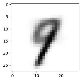
Now, Let’s see a reconstructed image created by our model.
1
2
3
4
5
6
7
8
9
10
11
i = 22
print("Low resolution")
plt.imshow(x_train[i],cmap=plt.cm.gray_r)
plt.show()
print("High resolution - Real")
plt.imshow(y_train[i],cmap=plt.cm.gray_r)
plt.show()
print("High resolution - From Model")
plt.imshow(x_reconstruction[i],cmap=plt.cm.gray_r)
plt.show()
Low resolution image:
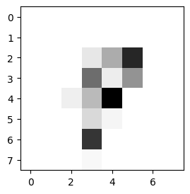
High resolution image real:
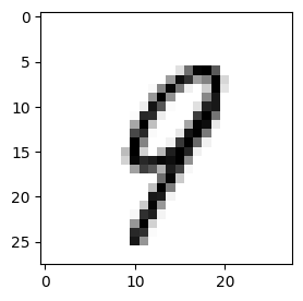
High resolution image created by the model:
Latent space
The latent space of a VAE refers to the space of the encoded variables that the model learns to represent the input data. Unlike traditional autoencoders, which map an input to a fixed representation, VAEs map an input to a distribution in the latent space. This means that the latent space is continuous, which means that nearby points in the latent space correspond to similar inputs in the data space.
Standar autoencoder latent space:
VAE latent space:
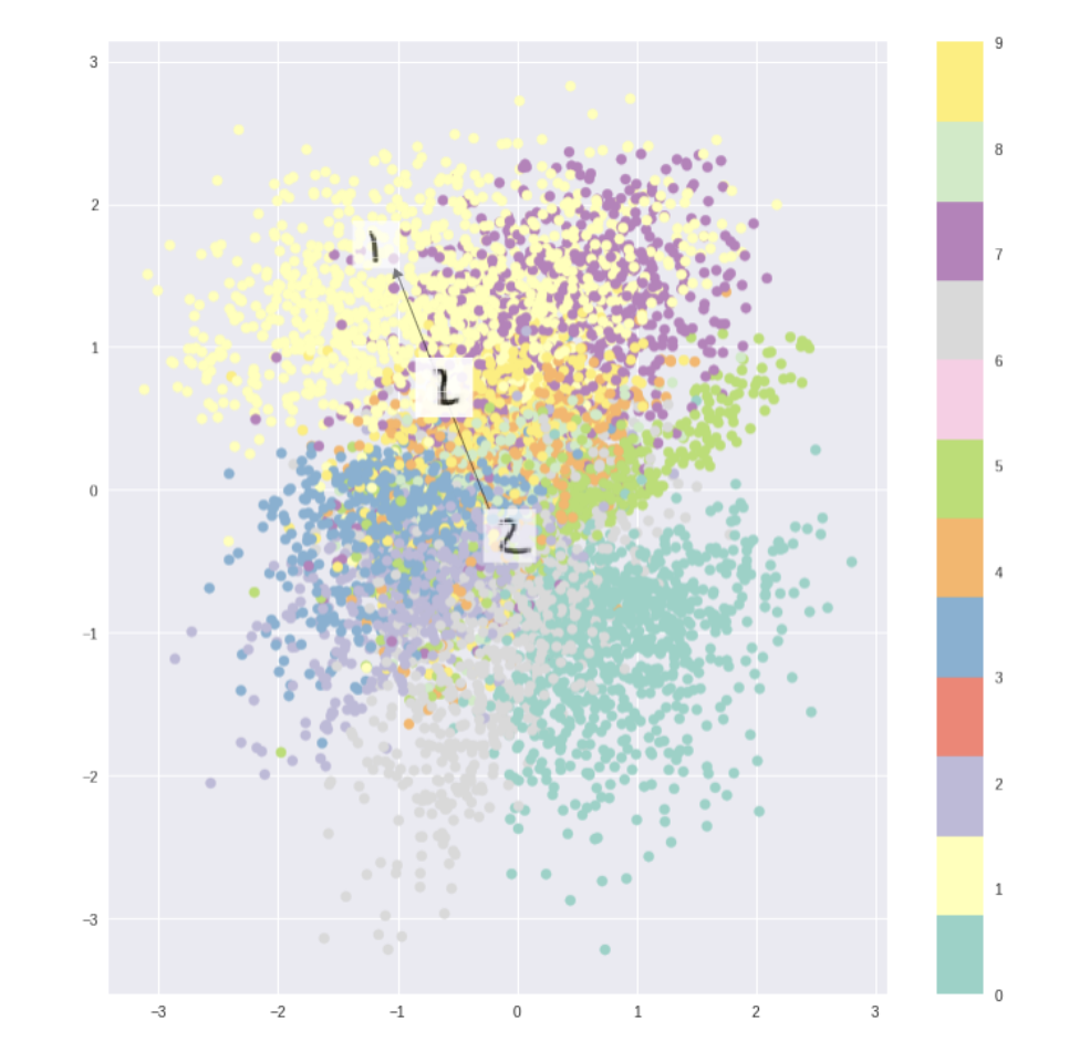
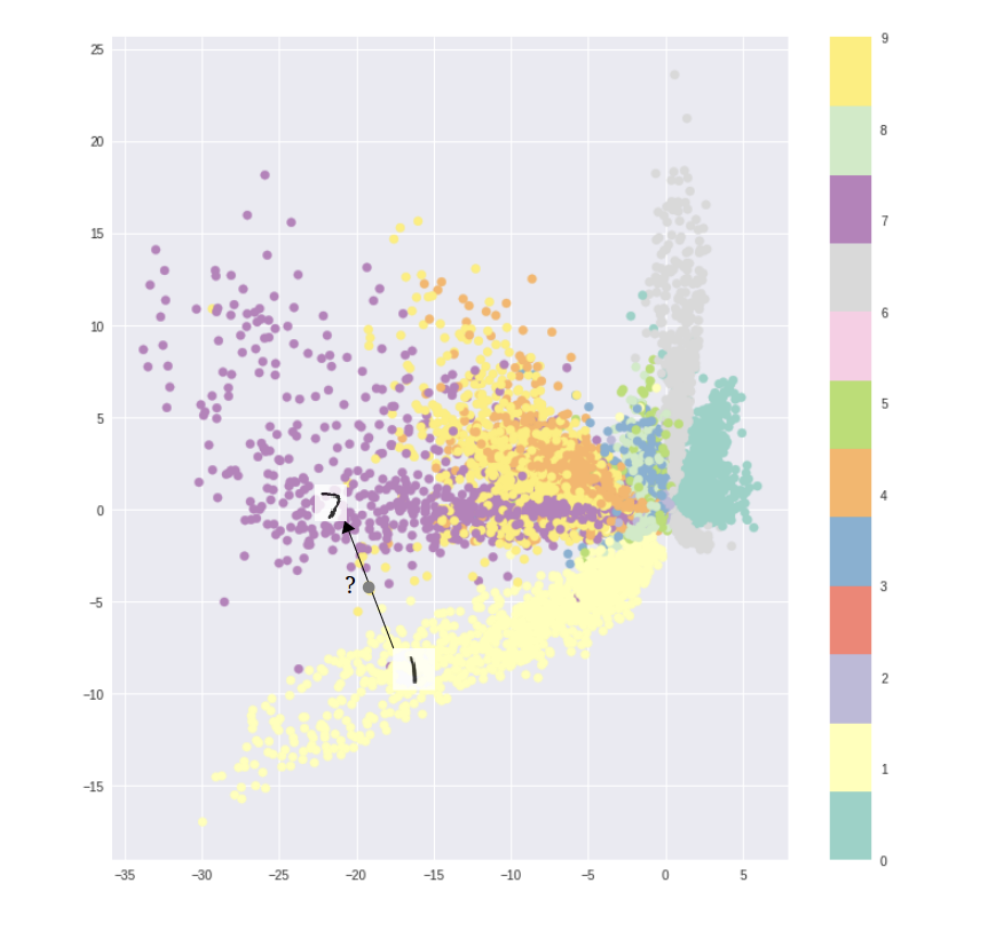
So, for standard autoencoders, we simply need to learn an encoding which allows us to reproduce the input. As you can see in the first figure, focusing only on reconstruction loss does allow us to reproduce the original handwritten digit, but there are areas in latent space which don’t represent any of our observed data. But, if we ensure that the latent distribution is continuos (through our KL loss) we can create a latent space similar to the second figure usefull for the image morphing.
Following a plot of some encoded data created by our model:
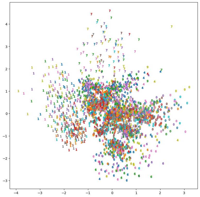
We can note that in the plot of the VAE’s learned latent space, similar digits are located closer together.
Morphing
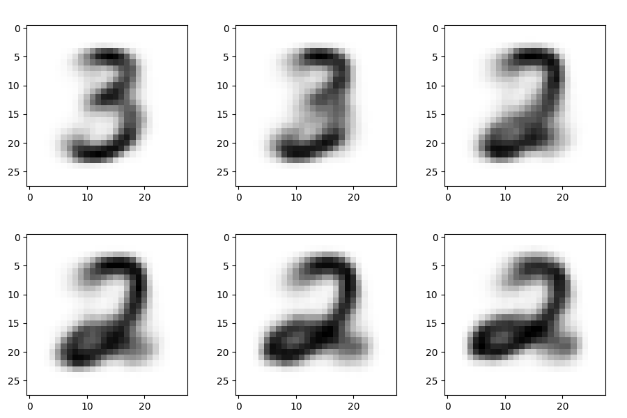
Now let’s dive in the last phase: morphing.
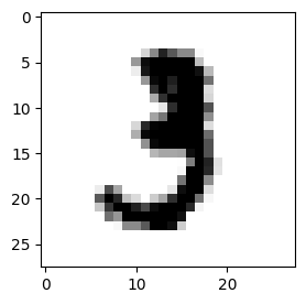
For example we want to morph the 3 digit with a 2 digit:
1
2
3
4
5
6
7
8
9
10
start=10
target=5
plt.rcParams['figure.figsize'] = [3, 3]


print("Start")
plt.imshow(y_train[start],cmap=plt.cm.gray_r)
plt.show()
print("Target")
plt.imshow(y_train[target],cmap=plt.cm.gray_r)
Start:
Target:
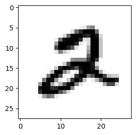
Now with the following code we take the latent space of the start image and target image, then we use the numpy linspace that return the evenly spaced numbers over a specified interval (in our case vector 2D). And then for each space we decode an image and then create a gif.
1
2
3
4
5
6
7
8
9
10
11
12
13
14
15
16
17
18
19
20
21
22
23
24
import imageio

x_encoded_start = x_encoded[start]
x_encoded_target= x_encoded[target]

filenames = []
STEP= 25

for img in np.linspace(x_encoded_start, x_encoded_target, num=STEP):
  reconstruction = vae.decoder.predict(img.reshape((1,2)))[0]
  plt.imshow(reconstruction,cmap=plt.cm.gray_r)
  i = len(filenames)
  filename = f'{i}.png'
  filenames.append(filename)

  plt.savefig(filename)
  plt.close()


# build gif
with imageio.get_writer('digitgif.gif', mode='I') as writer:
    for filename in filenames:
        image = imageio.imread(filename)
        writer.append_data(image)
Result of the morphing:
Reference link
For more details check out these links: