Hyperparameters
Have you ever tried tuning hyperparameters on a deep learning model? Finding the best hyperparameters is like find the right combination of parts and features that will make it run smoothly and look good (like pinping a car). But just like adding a spoiler or rims to your ride, hyperparameter tuning can be a bit of an art, and sometimes it feels like you’re just throwing random things at your model and hoping it sticks. In this blog post, we’ll take a look at some approach for hyperparameter tuning on deep learning models, and see if we can’t make your model as sleek and powerful as a tricked-out lowrider.

Panda vs Caviar


Nowadays thanks to the open-source tools it’s easy (more or less) to use deep learning models for real problem. For example, let’s imagine to solve the problem of classifying an image of Zalando’s article and for each image (the article) our software should guess the type (shoes, t-shirt etc.). Using keras (open-source) and a simple CNN model (that we can find easilly online) we can train the model reaching an accuracy of 90%. Also, if you don’t have computational power you can spend few dollars in cloud computing like databricks in ordert to train your model. Following the sample code used to train the Zalando dataset (fashion_mnist).
1
2
3
4
5
6
7
8
9
10
11
12
13
14
15
16
17
18
19
20
21
22
23
24
25
26
27
28
29
30
31
32
33
34
35
36
37
38
39
40
41
42
43
44
45
46
47
48
49
50
51
52
53
54
55
56
57
58
59
60
61
62
#Some imports
import numpy as np
import tensorflow as tf
from tensorflow import keras
from tensorflow.keras import layers
from tensorflow.keras.layers import Dense
from tensorflow.keras.models import Sequential

(x_train, y_train), (x_test, y_test) = keras.datasets.fashion_mnist.load_data()

#Simple pre processing of the data

# Scale images to the [0, 1] range
x_train = x_train.astype("float32") / 255
x_test = x_test.astype("float32") / 255
# Make sure images have shape (28, 28, 1)
x_train = np.expand_dims(x_train, -1)
x_test = np.expand_dims(x_test, -1)
print("x_train shape:", x_train.shape)
print(x_train.shape[0], "train samples")
print(x_test.shape[0], "test samples")

num_classes = 10
input_shape = (28, 28, 1)

# convert class vectors to binary class matrices
y_train = keras.utils.to_categorical(y_train, num_classes)
y_test = keras.utils.to_categorical(y_test, num_classes)

#function for the creation of the model
def create_model(n):
    kernel = int(n["kernel"])
    pool = int(n["pool"])
    model = keras.Sequential(
    [
        keras.Input(shape=input_shape),
        layers.Conv2D(n["first_conv"], kernel_size=(kernel, kernel), activation="relu"),
        layers.MaxPooling2D(pool_size=(pool, pool)),
        layers.Conv2D(n["second_conv"], kernel_size=(kernel, kernel), activation="relu"),
        layers.MaxPooling2D(pool_size=(pool, pool)),
        layers.Flatten(),
        layers.Dropout(n["dropout"]),
        layers.Dense(n["dense_1"], activation="relu"),
        layers.Dense(num_classes, activation="softmax"),
    ])
    return model

#Creation of the model and training
n = {
    "first_conv":32,
    "kernel":3,
    "pool":2,
    "second_conv":64,
    "dense_1":64,
    "dropout":0.5
}
model = create_model(n)
batch_size = 128
epochs = 15
model.compile(loss="categorical_crossentropy", optimizer="adam",metrics=["accuracy"])

model.fit(x_train, y_train, batch_size=batch_size, epochs=epochs, validation_split=0.2)
1
2
3
4
5
6
7
8
9
10
11
12
13
14
15
16
17
18
19
20
21
22
23
24
25
26
27
28
29
30
Epoch 1/15
375/375 [==============================] - 4s 5ms/step - loss: 0.6518 - accuracy: 0.7630 - val_loss: 0.4244 - val_accuracy: 0.8494
Epoch 2/15
375/375 [==============================] - 2s 4ms/step - loss: 0.4291 - accuracy: 0.8450 - val_loss: 0.3644 - val_accuracy: 0.8703
Epoch 3/15
375/375 [==============================] - 2s 4ms/step - loss: 0.3814 - accuracy: 0.8617 - val_loss: 0.3515 - val_accuracy: 0.8728
Epoch 4/15
375/375 [==============================] - 1s 4ms/step - loss: 0.3523 - accuracy: 0.8724 - val_loss: 0.3148 - val_accuracy: 0.8876
Epoch 5/15
375/375 [==============================] - 2s 4ms/step - loss: 0.3269 - accuracy: 0.8824 - val_loss: 0.3007 - val_accuracy: 0.8904
Epoch 6/15
375/375 [==============================] - 1s 4ms/step - loss: 0.3112 - accuracy: 0.8857 - val_loss: 0.2835 - val_accuracy: 0.8967
Epoch 7/15
 20/375 [>.............................] - ETA: 0s - loss: 0.2909 - accuracy: 0.893

*** WARNING: max output size exceeded, skipping output. ***

375/375 [==============================] - 2s 4ms/step - loss: 0.2702 - accuracy: 0.9009 - val_loss: 0.2714 - val_accuracy: 0.9003
Epoch 10/15
375/375 [==============================] - 1s 4ms/step - loss: 0.2623 - accuracy: 0.9032 - val_loss: 0.2512 - val_accuracy: 0.9075
Epoch 11/15
375/375 [==============================] - 1s 4ms/step - loss: 0.2520 - accuracy: 0.9077 - val_loss: 0.2580 - val_accuracy: 0.9046
Epoch 12/15
375/375 [==============================] - 1s 4ms/step - loss: 0.2470 - accuracy: 0.9083 - val_loss: 0.2548 - val_accuracy: 0.9066
Epoch 13/15
375/375 [==============================] - 2s 4ms/step - loss: 0.2382 - accuracy: 0.9118 - val_loss: 0.2414 - val_accuracy: 0.9109
Epoch 14/15
375/375 [==============================] - 2s 4ms/step - loss: 0.2300 - accuracy: 0.9150 - val_loss: 0.2400 - val_accuracy: 0.9102
Epoch 15/15
375/375 [==============================] - 1s 4ms/step - loss: 0.2292 - accuracy: 0.9145 - val_loss: 0.2431 - val_accuracy: 0.9111
Our simple model used in the example takes 6 parameters that define the convolution size, the dense neural network size, dropout and etc. In this blog post, I don’t want to discuss the CNN and the meaning of the defined model but about the process on How to choose these parameters? These parameters, also called hyperparameters, are an important part of deep learning model development and it’s not just for CNN but for ALL the deep learning models. Bigger is the model and more are the parameters.
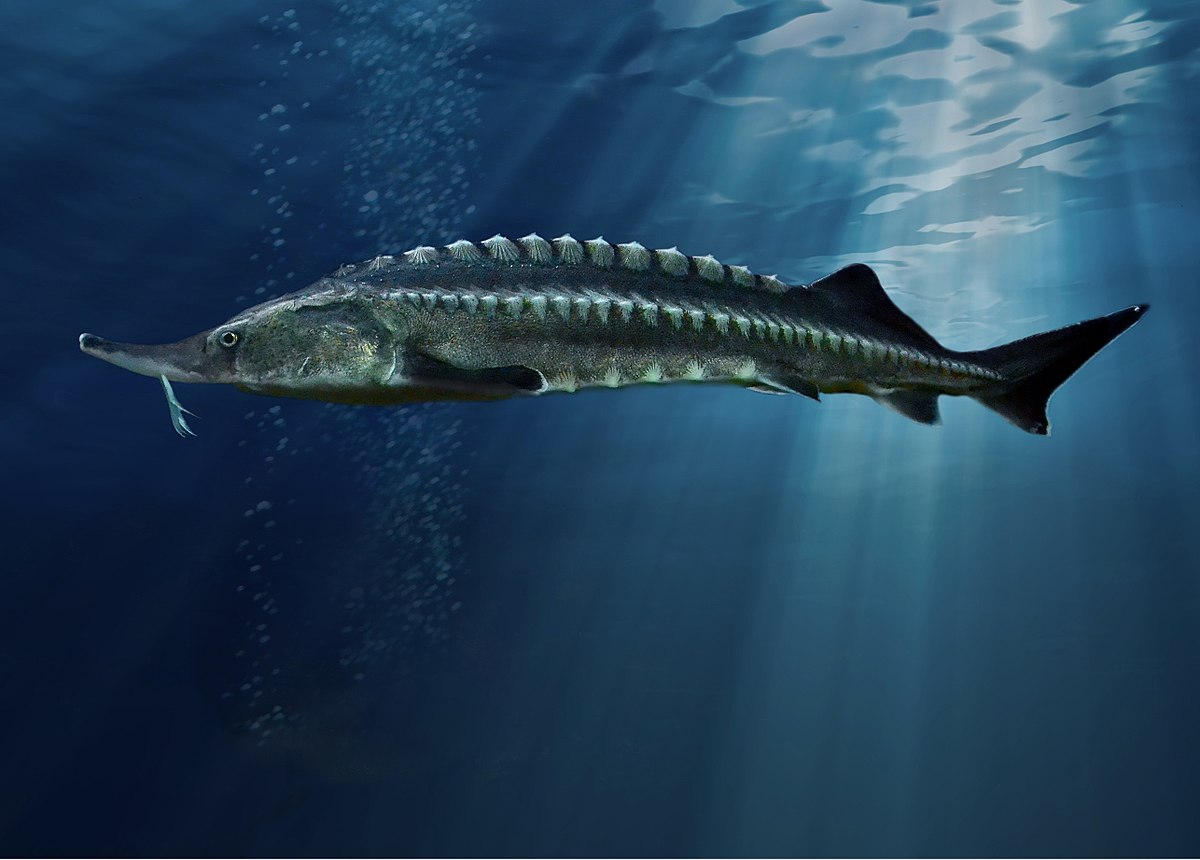
But, now the important question: Why panda vs caviar? In my experience, we have 2 ways to choose hyperparameters. The Panda way is when it is possible to train only a small number of models simultaneously. In this case, the developer babysit the model slowly. So for example we can increase in our example the dimension of the convolution layer and see if we can reach a better result. Then, try to modify the dropout threshold and so on. Another way, the caviar way, is to train several parallel models and just let it run on its own, even for multiple days, and then get the results and choose the best (like eggs of sturgeon fish). In this blog we will explore the second approch, the caviar way, using the cloud computing: Databrick.
Hyperopt
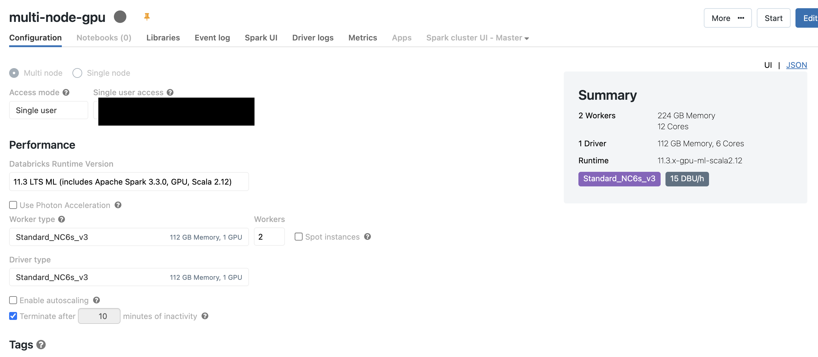
Databricks can be used also for Deep learning computing, creating easily GPU cluster with several workers with tensorflow, keras and others ML libraries.

In databricks you can train parallel models with Hyperopt library. With this approach, Hyperopt generates trials with different hyperparameter settings on the driver node, and each trial is executed from there, granting access to the full cluster resources. This approach works with any distributed machine learning algorithms or libraries, including Apache Spark MLlib. Hyperopt evaluates each trial on the driver node so that the machine learning algorithm itself can initiate distributed training.
Following code for finding the best parameters for our previous model:
1
2
3
4
5
6
7
8
9
10
11
12
13
14
15
16
17
18
19
20
21
22
23
24
25
26
27
28
29
30
31
32
33
34
35
36
37
38
39
40
41
42
43
44
45
46
47
48
49
50
51
from hyperopt import fmin, hp, tpe, STATUS_OK, SparkTrials, Trials
import mlflow
import mlflow.keras
import mlflow.tensorflow

def runNN(n):
  # Import tensorflow
  import tensorflow as tf

  # Log run information with mlflow.tensorflow.autolog()
  mlflow.tensorflow.autolog()

  model = create_model(n)

  # Select optimizer
  optimizer_call = getattr(tf.keras.optimizers, n["optimizer"])
  optimizer = optimizer_call(learning_rate=n["learning_rate"])

  # Compile model
  model.compile(loss="categorical_crossentropy",
                optimizer=optimizer,
                metrics=["accuracy"])

  history = model.fit(x_train, y_train, validation_split=.2, epochs=15, verbose=2)

  # Evaluate the model
  score = model.evaluate(x_test, y_test, verbose=0)
  obj_metric = score[0]
  return {"loss": obj_metric, "status": STATUS_OK}

#Adding also learning_rate and optimizer as parameters to test
space = {
  "first_conv": hp.choice("first_conv", [32,64]),
  "second_conv": hp.choice("second_conv", [32,64,128]),
  "kernel": hp.quniform("kernel", 3, 5, 2),
  "pool": hp.quniform("pool", 2, 3, 1),
  "dropout": hp.quniform("dropout", 0.3, 0.7, 0.1),
  "learning_rate": hp.loguniform("learning_rate", -5, 0),
  "dense_1": hp.choice("dense_1", [64,128,256]),
  "optimizer": hp.choice("optimizer", ["Adadelta", "Adam"])
 }

spark_trials = SparkTrials(3)

# Using mlflow to store all the results
with mlflow.start_run():
  best_hyperparam = fmin(fn=runNN,
                         space=space,
                         algo=tpe.suggest,
                         max_evals=50,
                         trials=spark_trials)
After the execution we can extract the best parameters:
1
2
import hyperopt
print(hyperopt.space_eval(space, best_hyperparam))
1
2
{'dense_1': 256, 'dropout': 0.4, 'first_conv': 32, 'kernel': 4.0, 'learning_rate': 0.5705611339889008, 'optimizer': 'Adadelta', 'pool': 2.0, 'second_conv': 128}
MLFlow
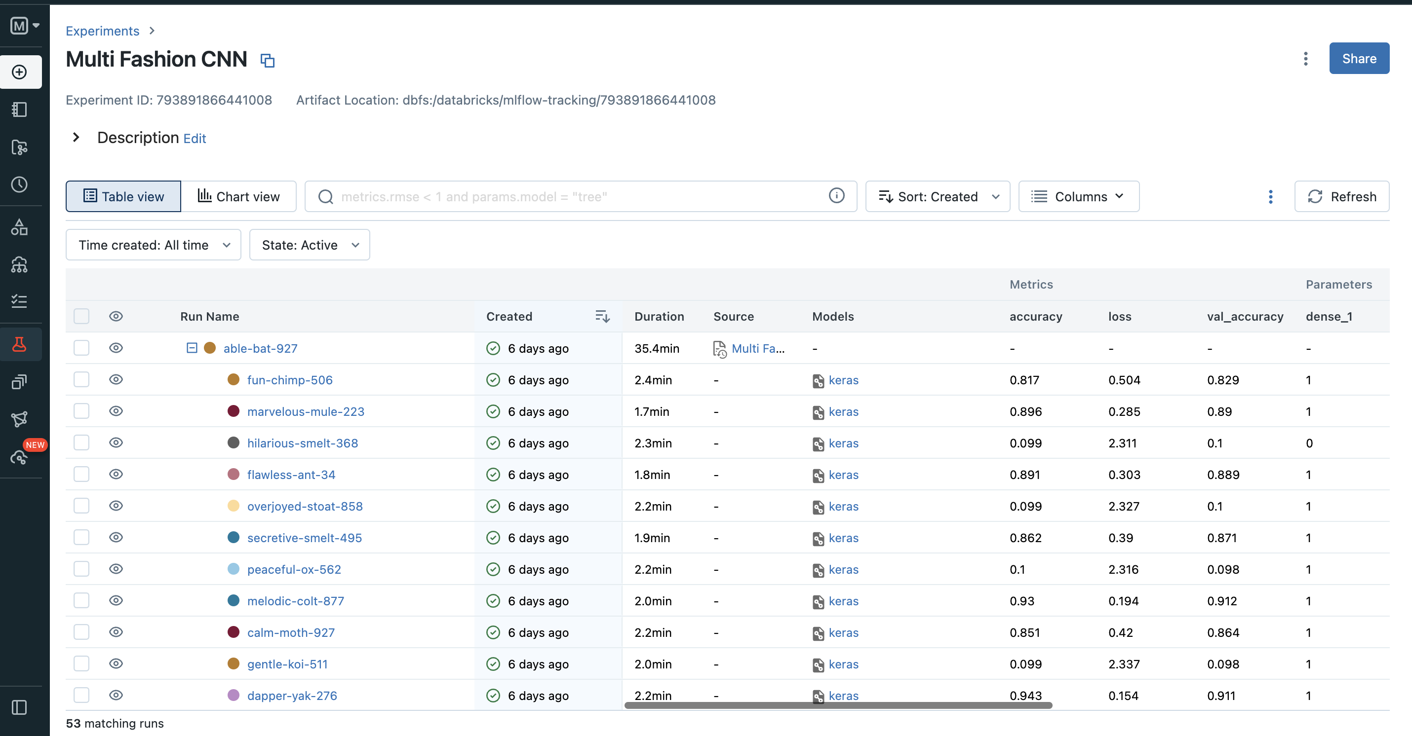
Using mlflow in our example we track our experiments, record the parameters and metrics of each run, and then easily compare the performance of different models. We can track our Experiments in databricks by changing the mode in Machine learning.

What this feature you can visualize the performance of each experiment using various charts, such as line plots, histograms, or scatter plots. You can also compare the hyperparameters of different runs and then select the best hyperparameters to focus on the next parallel training.
Reference link
For more details check out these links: