In the world of big data and data everywhere, streaming ETL is becoming increasingly prevalent.

Winter may be on the horizon, but so is an avalanche of data. Yet, fear not, for there’s a new champion in the arena – Delta Live Tables. Like heroes , DLT arrives to simplify your data ETL journey. So, grab your swords, or rather, your keyboards, as we embark on an epic journey to ‘simplify the stream’ with Delta Live Tables!
Delta Live Tables
Databricks Delta Live Tables is a simple framework for constructing robust, maintainable, and verifiable data processing pipelines. Instead of grappling with the intricacies of managing disparate Apache Spark tasks individually, Delta Live Tables provides a structured approach. Users are empowered to define streaming tables and materialized views, granting the system the responsibility of orchestrating data transformations as defined by user queries for each processing step.
Delta Live Tables datasets contain streaming tables and materialized views each with distinct processing characteristics:
- Streaming Tables: These tables process each record precisely once, rendering them well-suited for data sources following an append-only modality.
- Materialized Views: Designed to adapt dynamically, materialized views process records as necessary to furnish accurate results in accordance with the current data state. They are especially valuable for data sources subject to updates, deletions, aggregations, and change data capture processing (CDC).
The choice of dataset type should be guided by the specific requirements of your data processing workflows. Let’s deep dive into our first delta live table definition using python and Materialized Views.
Materialized view with DLT
In our first example let’s use the databricks sample wikipedia-datasets. The dataset contains counts of pairs extracted from the request logs of English Wikipedia. When a client requests a resource by following a link or performing a search, the URI of the webpage that linked to the resource is included with the request in an HTTP header called the “referer”. This data captures millions of pairs.
Delta Live Tables Python functions are defined in the dlt module, so let’s create a new Notebook and import dlt with others utilities modules:
1
2
3
import dlt
from pyspark.sql.functions import *
import random
In Python the @table decorator is used to define both materialized views and streaming tables and to define a materialized view we need to apply @table to a query that performs a static read against a data source.
1
2
3
4
5
6
7
json_path = "/databricks-datasets/wikipedia-datasets/data-001/clickstream/raw-uncompressed-json/2015_2_clickstream.json"

@dlt.table(
  comment="The raw wikipedia clickstream dataset, ingested from databricks-datasets."
)
def clickstream_raw():
  return (spark.read.format("json").load(json_path))
The previous code defines a Delta Live Table named clickstream_raw. It serves as the entry point for the raw Wikipedia clickstream dataset.
Now, we can prepare the dataset reading from the table clickstream_raw.
1
2
3
4
5
6
7
8
9
@dlt.table()
def clickstream_prepared():
  return (
    dlt.read("clickstream_raw")
      .withColumn("click_count", expr("CAST(n AS INT)"))
      .withColumnRenamed("curr_title", "current_page_title")
      .withColumnRenamed("prev_title", "previous_page_title")
      .select("current_page_title", "click_count", "previous_page_title")
  )
We can also dynamically generates multiple Delta Live Tables, for example generates multiple Delta Live Tables named clickstream_prepared_0, clickstream_prepared_1, and so on, up to a specified number.
1
2
3
4
5
6
7
8
9
10
11
12
13
14
15
16
17
TABLES_PREPROD = 3

def clickstream_prepared_rand(r: int):
  return (
    dlt.read("clickstream_raw")
      .withColumn("click_count", expr("CAST(n AS INT)"))
      .withColumnRenamed("curr_title", "current_page_title")
      .withColumnRenamed("prev_title", "previous_page_title")
      .filter(col("click_count") > r)
      .select("current_page_title", "click_count", "previous_page_title")
  )

for i in range(TABLES_PREPROD):
    @dlt.table(name=f"clickstream_prepared_{i}")
    def clickstream_prepared():
        r = random.randint(1,100)
        return clickstream_prepared_rand(r)
Each table is created with a different random threshold r for data filtering, ensuring diversity in the prepared datasets.
Lastly, we define a Delta Live Table called top_spark_referrers.
1
2
3
4
5
6
7
8
9
10
11
12
13
14
15
16
17
@dlt.table
def top_spark_referrers():
  df_join = None
  for i in range(TABLES_PREPROD):
    df = (
        dlt.read(f"clickstream_prepared_{i}")
        .filter(expr("current_page_title == 'Apache_Spark'"))
        .withColumnRenamed("previous_page_title", "referrer")
        .sort(desc("click_count"))
        .select("referrer", "click_count")
        .limit(10)
    )
    if df_join is None:
        df_join = df
    else:
        df_join = df_join.union(df)
  return df_join
This table aims to identify the top referrers to the “Apache_Spark” page from the prepared datasets. It iterates through the prepared tables, filters data related to “Apache Spark” selecting the top 10 referrers, and aggregates the results.
Upon finishing your notebook, we can configure our first DLT by:
- Naming Pipeline: Providing a meaningful name for your DLT pipeline.
- Choosing Pipeline Mode: Next, decide on the pipeline mode, which can be either “Trigger” or “Continuous.”
- Continuous Mode: In this mode, the pipeline operates continuously, processing new data as soon as it arrives. It’s like an ever-ready data processing engine, always prepared to handle incoming data.
- Trigger Mode: If you opt for “Trigger” mode, the pipeline operates in response to manual triggers or scheduled triggers that you specify. This gives you greater control over when the pipeline processes data, allowing you to synchronize it with your specific requirements.
- Specifying Notebook Paths: Indicate the paths of the notebooks that contain the code and configurations necessary for your DLT pipeline.
- Defining the Destination Path: One of the critical aspects of configuring your DLT is defining the destination path for your tables and associated metadata. This destination path can be a location in Databricks File System (DBFS) or cloud storage, depending on your infrastructure setup. Here’s why this step is pivotal: DLT’s materialized views and streaming tables are stored in Delta files within the destination path you specify. Delta files are the building blocks of data storage in DLT, ensuring durability and reliability for your processed data. By carefully defining this destination path, you’re effectively determining where your valuable data assets will reside, making it accessible for further analysis and insights.
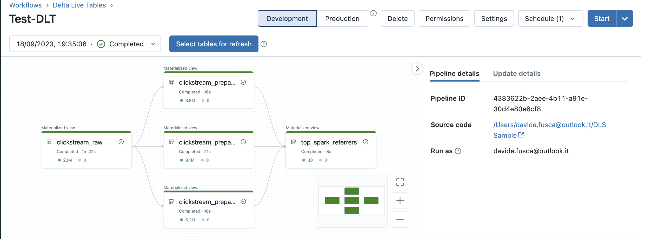
Delta Live Tables offers a user-friendly switch in its interface to manage the execution mode of your pipelines, allowing you to choose between development and production modes. This mode describe the following distinctions:
In Development Mode, the compute resources persist even after a successful or unsuccessful update. This feature enables you to efficiently reuse the same compute resources for subsequent updates of your pipeline without the delay of cluster initialization.
Auto Loader
Consider a scenario where you must handle numerous files within a continuously expanding folder, and your objective is to exclusively process newly added data. In such a situation, auto loader is the feature of DLT for you. With auto loader incrementally and efficiently processes new data files as they arrive in cloud storage without any additional setup. Auto Loader provides a Structured Streaming source called cloudFiles. Given an input directory path on the cloud file storage, the cloudFiles automatically processes new files as they arrive, with the option of also processing existing files in that directory.
Therefore for using auto loader we can just mount an Azure Data Lake Storage(or cloud storage) and redefine the function clickstream_raw:
1
2
3
4
5
6
7
8
@dlt.table()
def clickstream_raw():
    return (
        spark.readStream.format("cloudFiles")
        .option("cloudFiles.format", "json")
        .schema("curr_id INT, n INT, prev_title STRING, curr_title STRING, type STRING")
        .load("dbfs:/mnt/data/wiki-clickstream/")
    )
Let’s explore what it does step by step:
- spark.readStream.format(“cloudFiles”) indicates that you are setting up a streaming data source using the “cloudFiles” format. Then, clickstream_raw table will be a streaming table
- option(“cloudFiles.format”, “json”) sets the format of the data being read to JSON
- schema(“curr_id INT, n INT, prev_title STRING, curr_title STRING, type STRING”) defines the schema for the data you are reading
- load(“dbfs:/mnt/data/wiki-clickstream/”) specifies the path from which the data should be loaded. In this example, the path is the ADLS mounted in /mnt/data/.
Each time you introduce a new JSON file into the data lake, the next instance of triggering the Delta Live Table (DLT) will exclusively apply transformations to the new data. This prevents the unnecessary repetition of transformations on data that has already been processed.
Auto Loader in Databricks supports two modes:
Directory Listing Mode: Auto Loader identifies new files by listing the input directory. It’s easy to set up and doesn’t require complex permissions. It’s suitable for simple data processing tasks and can intelligently detect lexically ordered files.
File Notification Mode: This mode is ideal for large input directories or high file volumes. It uses cloud-based notification and queue services for efficient file event detection. However, it requires additional cloud permissions for setup.
Choose the mode that suits your specific data processing needs and infrastructure.
Streaming ETL with DLT
Delta Live Tables (DLT) is an ETL framework that efficiently manages streaming data, making it an ideal choice for various use cases, including those demanding real-time insights. DLT excels in low-latency streaming data pipelines, enabling rapid ingestion from event buses like Apache Kafka, AWS Kinesis, Azure Event Hubs and etc. In this section, we’ll use DLT with Apache Kafka, offering Python code to facilitate stream ingestion.
Azure function producer

To establish a Kafka service in Azure, we need to create of an Apache Kafka service within Confluent Cloud, accessible through your Azure subscription. Microsoft has collaborated with Confluent Cloud to streamline this experience, offering an integrated provisioning layer that bridges Azure to Confluent Cloud. This integration simplifies the management of Confluent Cloud within your Azure environment, ensuring a unified and seamless experience. Once your Confluent Cloud organization is established within your subscription, you can access the Confluent portal. From there, you can proceed to configure a Kafka cluster tailored to your specific needs, including creation of topics. For more detailed information, please refer to the provided resource links.
After the Kafka service setup is complete, the next step involves the creation of an Azure Key Vault. Within this Key Vault, you can securely store the API credentials required for establishing a connection to the Kafka service. This ensures that sensitive information remains protected and accessible only to authorized users and applications.
We are now prepared to develop a producer component. To achieve this, we will craft an Azure Python serveless application function. This function’s primary role is to transmit events to a Kafka topic. It will be triggered via an HTTP request, and its operation involves reading secure credentials from Azure Key Vault (connected via a user-managed service principal). Subsequently, the function will populate the Kafka topic with customer reviews extracted from a JSON file. This file serves as a sample dataset encompassing beauty customer reviews, including attributes such as text, reviewer details, and ratings.
For more info of the azure function you can navigate the folder Azure Function in github repository
Streaming Tables with DLT
We can now proceed to create the Delta Live Table (DLT) responsible for data ingestion, which involves reading data from Kafka.Let’s break down:
1
2
3
4
5
6
7
8
9
10
11
12
13
14
15
@dlt.table()
def rating_raw():

    return (
        spark.readStream
        .format("kafka")
        .option("kafka.bootstrap.servers", spark.conf.get("kafka.bootstrap.servers"))
        .option("kafka.sasl.mechanism", "PLAIN")
        .option("kafka.security.protocol", "SASL_SSL")
        .option("kafka.session.timeout.ms", "45000")
        .option("kafka.sasl.jaas.config", "kafkashaded.org.apache.kafka.common.security.plain.PlainLoginModule required username='{}' password='{}';".format(dbutils.secrets.get("function-scope","KAFKA-ID"), dbutils.secrets.get("function-scope","KAFKA-KEY")))
        .option("subscribe", spark.conf.get("kafka.subscribe"))
        .option("startingOffsets", "latest")
        .load()
    )
This table is responsible for ingesting raw data from a Kafka source. It uses the Kafka data source format and specifies various Kafka-related options, including the bootstrap servers, security (username and password), and subscription topic.
1
2
3
4
5
6
7
8
9
@dlt.table()
def rating_preproc():
    schema = "overall DOUBLE, verified BOOLEAN, reviewText STRING, reviewerName STRING"

    return (
        dlt.read("rating_raw")
        .select(from_json(col("value").cast("string"), schema ).alias("data"))
        .select("data.overall","data.verified","data.reviewText","data.reviewerName")
    )
The rating_preproc table preprocess the ingested data. It parse the json data and selects specific fields from the parsed JSON data, including “overall” (rating), “verified,” “reviewText” (review content), and “reviewerName” (reviewer’s name).
1
2
3
4
5
6
7
8
9
10
11
12
13
@dlt.table()
def reviewer_score():

    return (
        dlt.read("rating_preproc")
        .select("overall","reviewerName")
        .filter(col("overall").isNotNull() & col("reviewerName").isNotNull())
        .groupby("reviewerName").agg(
            count("reviewerName").alias("count_review"),
            avg("overall").alias("score")
        )
        .orderBy(col("count_review").desc())
    )
reviewer_score table computes reviewer scores by reading the preprocessed data and select the “overall” (rating) and “reviewerName” columns. It filters out rows where either the rating or reviewer’s name is null, groups the data by reviewerName, and aggregates statistics, including the count of reviews and the average score for each reviewer. The results are ordered by the number of reviews in descending order.
1
2
3
4
5
6
7
8
9
10
11
12
13
14
15
16
@dlt.table()
def top_review():
    return (
        dlt.read("rating_preproc")
        .select("overall","reviewerName","reviewText")
        .filter(col("overall").isNotNull() & col("reviewerName").isNotNull() & col("reviewText").isNotNull())
        .orderBy(col("overall").desc())
    )
@dlt.table()
def worst_review():
    return (
        dlt.read("rating_preproc")
        .select("overall","reviewerName","reviewText")
        .filter(col("overall").isNotNull() & col("reviewerName").isNotNull() & col("reviewText").isNotNull())
        .orderBy(col("overall").asc())
    )
The tables top_review and worst_review focuses on retrieving the top-rated reviews and the worst-rated reviews.
To automate the execution of both the function and the Delta Live Table (DLT), I’ve set up a straightforward pipeline using Azure Data Factory. This pipeline initiates the Azure function trigger, followed by the triggering of the DLT process in Databricks.

Dashboard Streaming Data
Following the definition of your Delta Live Table (DLT), another fascinating aspect to explore is data visualization. As mentioned earlier, DLT stores data in the Delta format within the designated folder specified during DLT creation. This data can be visualized exporting the data to Business Intelligence (BI) tools like PowerBI for comprehensive visualization and analysis. Alternatively, you can leverage Databricks Dashboard and SQL capabilities for visualization. To enable Databricks Dashboard, you must first activate the Unity Catalog. Once enabled, you can craft custom SQL queries to access data from your DLT table and subsequently visualize it using Databricks Dashboard. This empowers you to create interactive and insightful data visualizations directly within the Databricks environment.
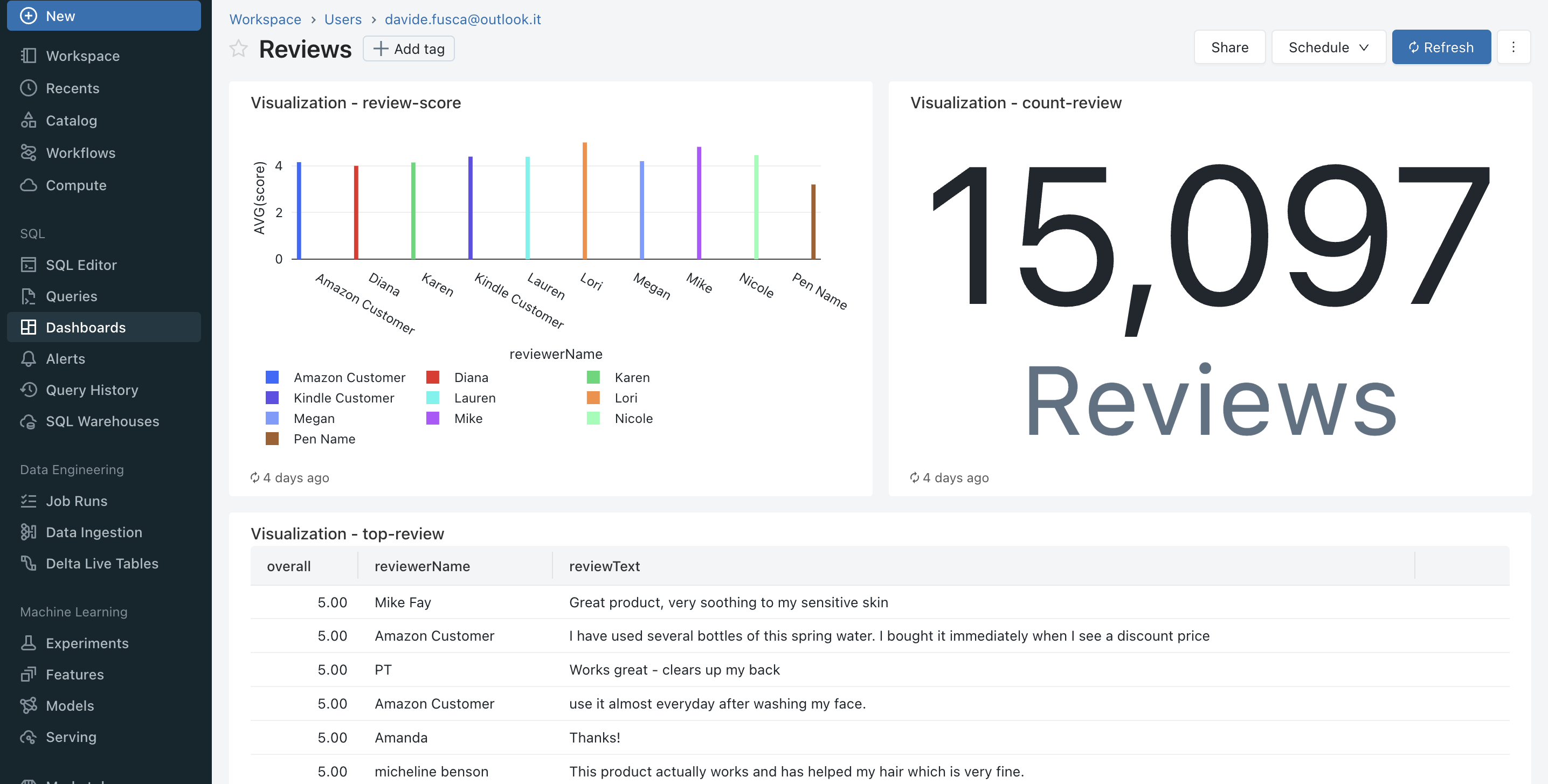
The dashboard shown above has been generated using the data populated by the previously defined Delta Live Table (DLT).
NOTE: By utilizing Databricks SQL queries, you can use the power of serverless compute. Databricks enables you to create serverless SQL warehouses, which offer immediate compute resources and are efficiently managed by the Databricks. These serverless SQL warehouses utilize compute clusters within your Databricks account. This provides you with the flexibility and scalability to execute your SQL queries effectively within the Databricks environment.
For more info you can find all the Notebooks and Azure Function in github repository

Reference link
For more details check out these links:
Databricks orchestration from ADF