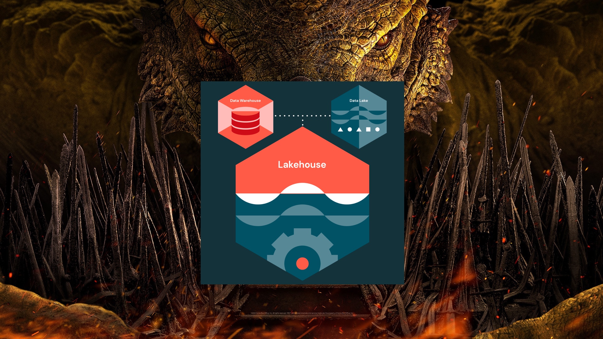
Data warehouse vs Data Lake
Data lakes exist in response to the high limitations of data warehouses. While DW provide highly performant and scalable analytics, they are expensive and can’t handle the modern use cases (like machine learning). Data lakes are a single, central location, where it can be saved without the need to impose a schema (you can store structured and unstructured data). Data lake, unlike most databases and data warehouses, can process all data types (like images, video, audio and documents) with open formats and scales with low cost which are critical for today’s machine learning use cases.
| Data lakes | Data warehouses | |
|---|---|---|
| Format | Open | Closed, proprietary |
| Cost | Low ($) | High ($$$) |
| Data | Structured and unstructured | Structured |
| Scalability | Low cost | Exponentially expensive |
| Reliability | Low quality | High quality |
The born of LakeHouse
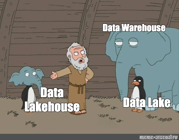
Despite the pros of data lake its lack of some critical features:
Reliability: data reliability is a major issue of the data lake and makes it difficult for data scientists and analysts to reason about the data. For example when someone is writing data into the data lake, but because of a hardware or software failure, the write job does not complete. In this scenario, data engineers must spend time and energy deleting any corrupted data. Also, deletion and update of data are incredibly difficult to perform because transactions do not exist and there is no mechanism to ensure data consistency.
Slow performance: holding millions of files and tables require your query engine must be optimized for performance at scale. For example having a large number of small files in a data lake can slow down performance or repeatedly accessing data from storage without caching slow your query performance.
The answer to the challenges of data lakes is the lakehouse, which adds a transactional storage layer on top: which means that every operation performed on it is atomic (it will either succeed completely or fail completely). Also, lakehouse improves query performance thanks to several optimization techniques like small file compaction, caching and indices.
In the following sections we will explore data lake and lakehouse in our favorites big data platform: Databricks
Data object in databricks
There are five primary objects in the Databricks:
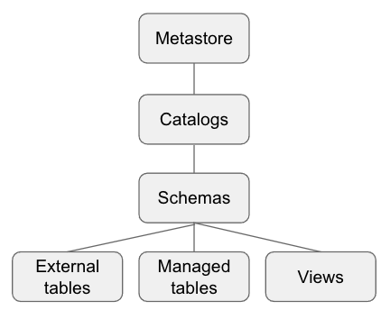
Metastore: contains all of the metadata that defines data objects in Databricks. Exist 3 type of metastore: Unity catalog (share metadata across multiple Databricks), Hive metastore (built-in Hive metastore and each cluster securely accesses metadata from a central repository) and External metastore (bring your own metastore to Databricks)
Catalog: group of schemas. Catalogs exist as objects within a metastore.
Schema or database: collection of data objects, such as tables or views.
Table: collection of rows and columns stored as data files.
View: saved query typically against one or more tables.

Managed Table
Let’s load data from CSV files using the following command:
1
2
3
4
df = (spark.read.option("header",True)
                .option("delimiter","|")
                .csv(path)
     )
Now we can try to create a table into the metastore:
1
df.write.format("csv").saveAsTable("sales")
In this example we are reading and writing csv files but you can easily apply the same code replacing csv(path) and format(“csv”) with other formats (parquet, json, etc.)
We can check the details of the created table with the command:
1
DESCRIBE TABLE EXTENDED sales;
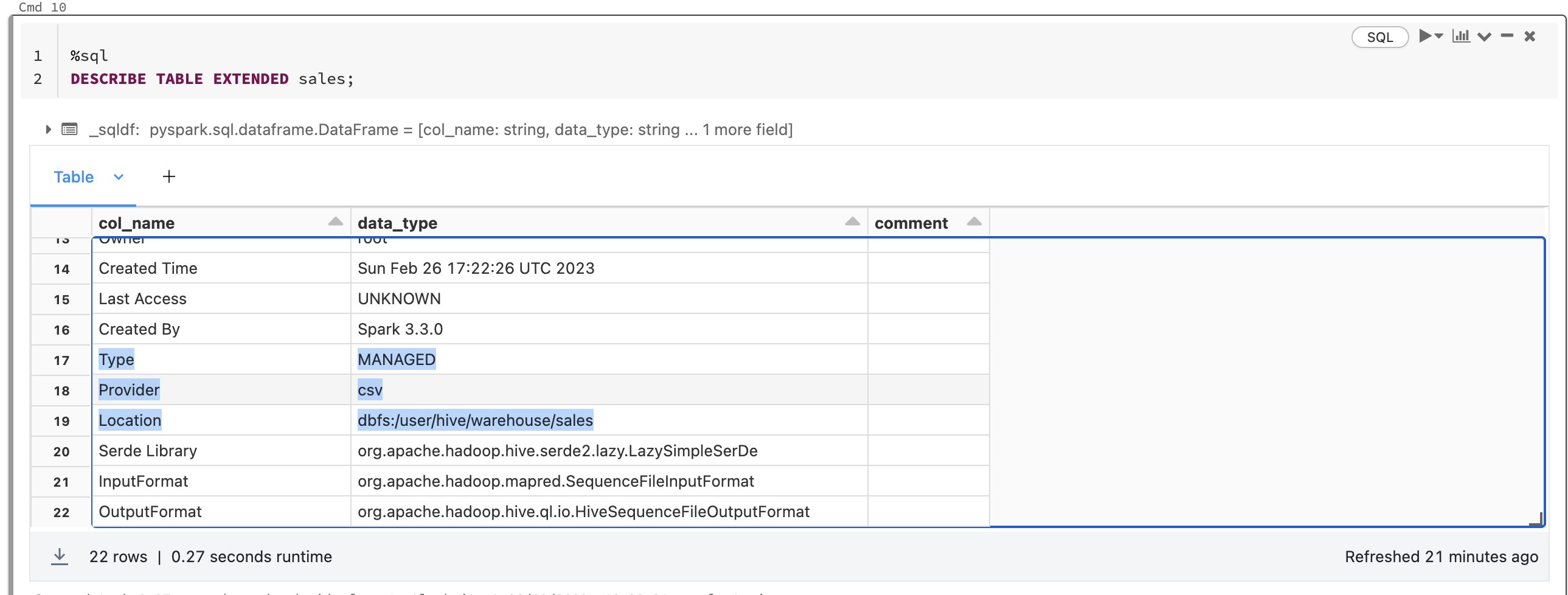
Managed tables are the default way to create tables databricks and are stored in the root storage location you configured when you created the metastore.
After the successful creation of a table is possible to load data with the command:
1
df = spark.table("sales")
With a managed table, the underlying directories and data get wiped out when the table is dropped.
Indeed after the execution of the command we delete also the related files:
1
2
%sql
DROP TABLE IF EXISTS sales;

External Table
For creating an external table we have to specify an output path:
1
df.write.format("csv").option("path","dbfs:/FileStore/tables/sales").saveAsTable("sales")
We can display the details of the previous created table:
1
DESCRIBE TABLE EXTENDED sales;
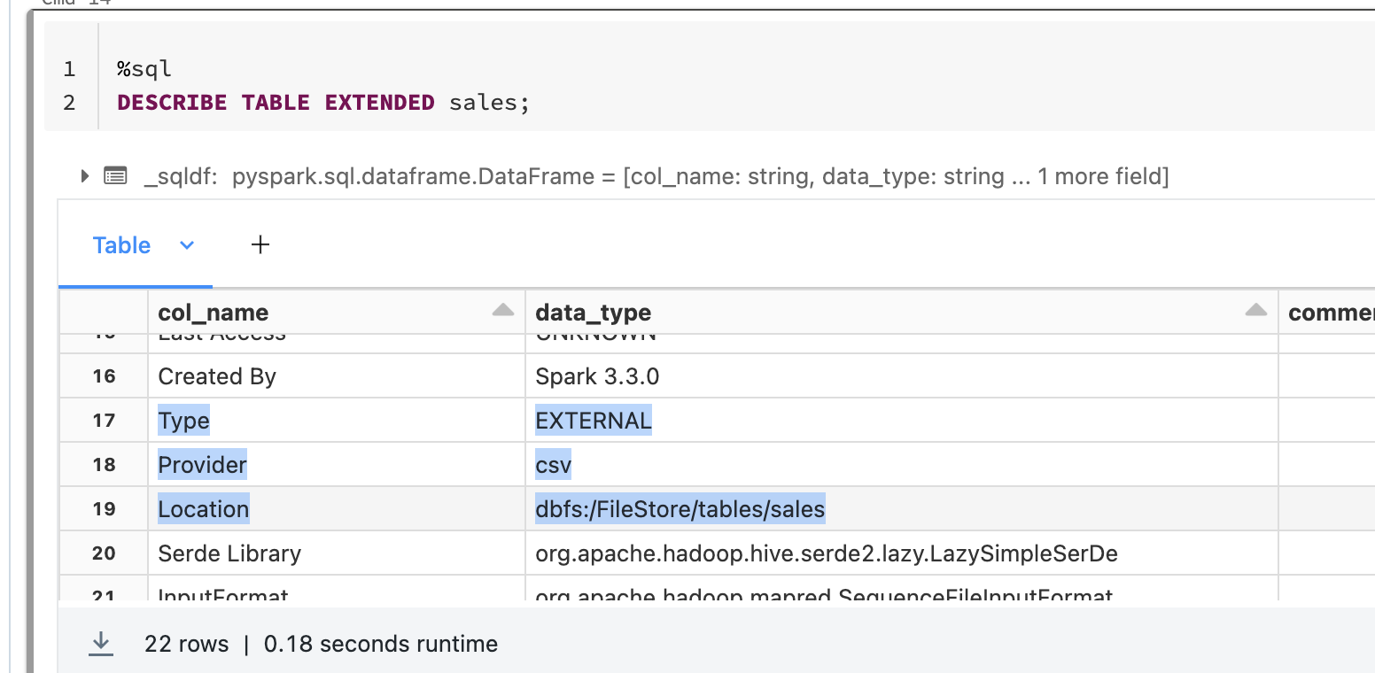
Now if we try to delete the table the files still exist.
1
2
%sql
DROP TABLE IF EXISTS sales;

View
If you don’t want to create table writing files you can use view:
1
df.createOrReplaceTempView("sales_view")
Then you can load the view using the same command for reading tables:
1
df = spark.table("sales_view")
A view is a read-only object composed from one or more tables and views in a metastore. A view can be created from tables and other views in multiple schemas and catalogs.
A normal View is available across the context of a Notebook. If you want to make avaliable to all the Notebooks then you can use the: Global View.
1
df.createOrReplaceGlobalTempView("sales_view")
Delta lake
Delta Lake is an open-source storage framework that enables building a Lakehouse. Delta Lake is the default storage format for all operations on Databricks. Let’s create a delta table:
1
2
3
4
5
df = (spark.read.option("header",True)
                .option("delimiter","|")
                .csv(path)
     )
df.write.format("delta").option("path","dbfs:/FileStore/delta-tables/sales").saveAsTable("raw_sales")
If we print content of the folder delta-tables we can see that delta format basically extends Parquet data files with a file-based transaction log (json log file) for ACID transactions.
1
dbutils.fs.ls("dbfs:/FileStore/delta-tables/sales")
1
2
3
4
5
6
7
8
9
Out[5]: [FileInfo(path='dbfs:/FileStore/delta-tables/sales/_delta_log/', name='_delta_log/', size=0, modificationTime=1677952173000),
 FileInfo(path='dbfs:/FileStore/delta-tables/sales/part-00000-8c601529-a08b-4502-8768-5b860d40a073-c000.snappy.parquet', name='part-00000-8c601529-a08b-4502-8768-5b860d40a073-c000.snappy.parquet', size=112431, modificationTime=1677952164000),
 FileInfo(path='dbfs:/FileStore/delta-tables/sales/part-00001-cccf4b0d-e905-406f-99dc-ec49a271c230-c000.snappy.parquet', name='part-00001-cccf4b0d-e905-406f-99dc-ec49a271c230-c000.snappy.parquet', size=106406, modificationTime=1677952164000),
 FileInfo(path='dbfs:/FileStore/delta-tables/sales/part-00002-9e2b5b02-df33-44a3-b998-c77214cea9ce-c000.snappy.parquet', name='part-00002-9e2b5b02-df33-44a3-b998-c77214cea9ce-c000.snappy.parquet', size=98891, modificationTime=1677952164000),
 FileInfo(path='dbfs:/FileStore/delta-tables/sales/part-00003-733e567b-d553-4dd8-a32e-55b4333d1dda-c000.snappy.parquet', name='part-00003-733e567b-d553-4dd8-a32e-55b4333d1dda-c000.snappy.parquet', size=64951, modificationTime=1677952164000)]

 Out[6]: [FileInfo(path='dbfs:/FileStore/delta-tables/sales/_delta_log/00000000000000000000.crc', name='00000000000000000000.crc', size=6557, modificationTime=1677952173000),
 FileInfo(path='dbfs:/FileStore/delta-tables/sales/_delta_log/00000000000000000000.json', name='00000000000000000000.json', size=5637, modificationTime=1677952165000),
 FileInfo(path='dbfs:/FileStore/delta-tables/sales/_delta_log/__tmp_path_dir/', name='__tmp_path_dir/', size=0, modificationTime=1677952173000)]
Time travel
Time travel capabilities are one of the most used capabilities of delta format. As we see in the previous example Delta Lake stores data in Parquet files and information about transactions in the _delta_log metadata folder.
The _delta_log metadata folder tracks the Parquet data files that are added and removed from the Delta table for each transaction.
So, let’s insert some data:
1
2
3
4
5
spark.sql("""
INSERT INTO raw_sales VALUES (1,'test',00000,1,20.0,1,null)
""")

df.write.format("delta").option("path","dbfs:/FileStore/delta-tables/sales").mode("append").save()
Now, each time you write the delta table you create a new version of the table:
1
2
%sql
DESCRIBE HISTORY raw_sales

And you can retrieve a DataFrame from a Delta table with a specific version of the table:
1
df1 = spark.read.format('delta').option('versionAsOf', 1).table("raw_sales")
or, alternately:
1
df1 = spark.read.format('delta').option('timestampAsOf', '2023-03-05').table("raw_sales")
Optimization
Once you have performed multiple changes to a table, you might have a lot of small files. Another important feature of delta is the OPTIMIZE feature to collapse small files into larger ones to improve the speed of queries :
1
OPTIMIZE raw_sales
Or :
1
2
3
from delta.tables import *
deltaTable = DeltaTable.forPath(spark, "dbfs:/FileStore/delta-tables/sales")
deltaTable.optimize().executeCompaction()
Partitioning data is one of the most used optimization in data lake for physically splits the data into different files/directories having only one specific value. Partitioning is useful when there are not so many possible values and can improve the speed of read queries. Data partitioning in Spark generally works great for dates or categorical columns, it is not well suited for high-cardinality columns and this is where it comes into play ZOrder. ZOrder provides clustering of related data inside the files that may contain multiple possible values for given columns. This dramatically reduce the amount of data that needs to be read:
1
2
OPTIMIZE raw_sales
ZORDER BY (email)
Bronze, Silver and Gold
The most common pattern we see in data lake is to collect real-time streaming data and save it into inexpensive, cloud storage like Blob storage or S3 buckets. As a result, we tend to have a lot of raw, unstructured data from various sources and adding structure to the data so that it can be fed into machine learning models it easily become convoluted and unorganized data lakes: data swamps.
Delta lake solve this dilemma with the following architecture:

In the beginning you can easily convert your existing data tables from whatever format they are currently stored in (CSV, Parquet, etc.) and save them as a Bronze table. The goal of bronze table is to maintains the raw state of the data source and append new data incrementally and grows over time. Bronze table in essence acts as a landing zone for your data but is far from useful in its current form. It requires significant cleaning, transformation, and structure before it can be used. So, after performing ETL we can save the cleaned and processed data to a new Delta Silver table, which allows us to save the result as a new table without modifying our original data (Bronze table). Finally, the Gold table is highly refined and aggregated data, containing data for analytics and machine learning. In general, because aggregations, joins, and filtering are handled in this stage, users of gold table see low latency query performance on data in this tables.
The reason of the existence of silver table and why we don’t simply connect Gold tables directly to Bronze tables is that it would cause a lot of duplicated effort. That would require each business unit to perform the same ETL on their data.
Reference link
This page describes a brief introduction to the world of lakehouse and delta lake. For more details check out these links: